Liquidity refers to the degree to which an asset or security can be quickly bought or sold in the market without affecting the asset’s price. High liquidity means transactions can be conducted smoothly and with minimal price disturbance. Conversely, low liquidity often means that buying or selling an asset could significantly affect its price due to a lack of willing buyers or sellers.
In the financial markets, liquidity can be characterized by a high level of trading activity. Assets that can be easily bought or sold are known as liquid assets. These assets can include certain stocks and bonds, commodities, currencies, and money market instruments. The most liquid asset is cash, which can be readily exchanged for goods, services, or other assets.
On the other hand, the real estate market is an example of a relatively illiquid market because assets (properties) can’t be easily or quickly converted into cash without potentially altering the asset’s price significantly. Large capital goods, such as production machinery, are also relatively illiquid.
Regarding monetary policy, liquidity provided by central banks often refers to the money supply in the economy. Central banks use various tools to influence this liquidity, including adjusting interest rates and reserve requirements or through open market operations (buying or selling securities). These tools can influence the ease with which banks lend money, ultimately affecting economic activity.
In times of financial stress, central banks can act as a ‘lender of last resort,’ providing liquidity to institutions to keep the financial system functioning. This can be crucial in preventing or mitigating financial crises when normal liquidity channels can dry up, leading to a severe contraction in economic activity. This was seen in actions by central banks during the 2008 financial crisis and, more recently, during the COVID-19 pandemic, when central banks around the world injected large amounts of liquidity into their respective economies to keep them functioning.
How do we define liquidity?
Liquidity provided by central banks through money supply is the most critical liquidity that exists and strongly affects liquidity on a micro level. However, the exact definition of liquidity varies greatly, and you will find many examples of how liquidity measures are calculated. In this blog, I will take you through our definition of liquidity, what it means, and how we can use data from central banks to create an indicator that can estimate the current liquidity development.
We utilize a variable called M1, which is the narrow money supply central banks publish regularly. M1 includes all physical money, such as coins and currency, as well as demand deposits, checking accounts, and other liquid and near-liquid assets that can be quickly converted into cash. M1 is a narrow measure of money’s function as a medium of exchange; it excludes more complex financial assets and longer-term investments. Historically, narrow money growth leads to changes in economic growth, which is why we are using that as the basis for our liquidity indicator. Since we are interested in the effect of liquidity on real economic development, we will deflate the time series with the change in the consumer price index (inflation). The formula for liquidity becomes the following:
Liquidity = Yearly change in M1 (narrow money supply) – Yearly change in consumer price index (inflation)
Liquidity and the economic effects
We have shown the close relationship between changes in the liquidity measure and the economy below:
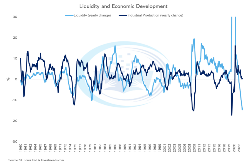
The graph is capped between +30% and -30% to provide a better graphical representation of the relationship between the change in liquidity and economic development. Here we use industrial production as the proxy for economic growth. There are a couple of reasons why this is the case, one of them being that industrial production is closely related to the manufacturing side of the economy, which generally is the most cyclical part. There is a historical relationship between changes in industrial production and a country’s output (GDP). Also, industrial production is a monthly measure, which helps align with the frequency of the liquidity indicator.
Just by eyeballing the chart, we can see that when liquidity falls, this usually leads to a fall in economic development. However, liquidity may also be leading the change in economic development. What we mean by this is that when liquidity changes, we will see economic changes a few months later. I won’t go into detail with this (it may be for a different blog), but statistically, a cross-correlation analysis reveals that the optimal lag period is 12 months. The data comes from St. Louis Fed and the following keywords:
- CPIAUCSL = Consumer Price Index (Index)
- M1SL = M1 Money Supply (Index)
- INDPRO = Industrial Production (Index)
Liquidity and the financial effects
Our liquidity indicator works well at anticipating turns in economic development. But to help anticipate changes in the financial markets, we must make a critical assumption. We must assume that some of the liquidity is used for economic purposes. At the same time, the rest (excess) flows directly into the financial markets. This is the reason we are calling this the excess liquidity indicator:
Excess Liquidity = Real Money Growth (Liquidity) – Economic Growth
An easy way to visualize the impact of excess liquidity on the financial markets is by graphing out our new excess indicator and the yearly change in the S&P 500.
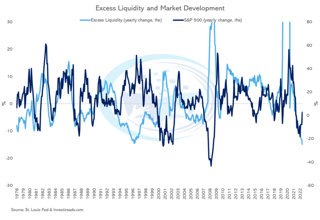
Again, just by eyeballing the chart, we can see that when excess liquidity falls, this usually leads to a fall in the development of the S&P 500. Again, I won’t go into detail with this, but statistically a cross-correlation analysis reveals that the optimal lag period is 9 months. Therefore, a change in the excess liquidity change can be used as a forewarning in terms of the stock market’s direction. This is neat since we can start collecting these indicators to help guide our investment decisions (using them tactically to avoid losing money).
We can see the same pattern in more economically sensitive sectors of the economy, in this case, the US Small Caps (Russell 2000). Here it is shown together with the excess liquidity indicator.
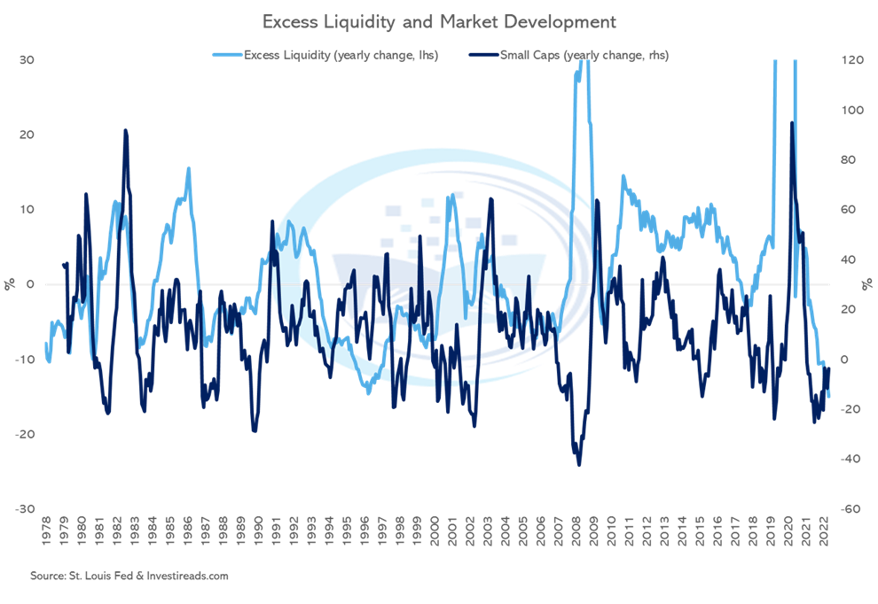
Even more interesting is that the excess liquidity indicator is leading the change in small caps by 7-8 months, and the lead is much more pronounced than with the change in the S&P 500. This is excellent information if we want to know periods when we can expect higher or lower equity returns with the intent of using this information for tactical purposes.
Conclusion
In this blog, I have shown you how to define liquidity and use data to approximate the liquidity situation. I must address that liquidity is a complex term with different ways of approximating it. However, the key message is that economic development nowadays is driven by financial flows in the form of savings and credits (money supply), which makes it essential to follow this very closely. I have provided an easier way of doing this, but more accurate and complex methods exist. Here I need to mention the book “Capital Wars – The Rise of Global Liquidity” which is fantastic work by Michael J. Howell. I have provided a link to this through the picture below. As a disclaimer, it is worth mentioning that the book is not an easy read for novice investors. But at some point in your financial education, I strongly recommend reading this book, as it keeps getting more and more critical.